Jet Engine Fault Detection
We created unsupervised LSTM autoencoder models to leverage the temporal nature of NASA jet engine data. We processed the data to remove sensors with no pertinent features, trimmed degradation data to only train on healthy, pre-fault bahvior, and normalized the data for model stability. We use K-Clustering to cluster by flight operating regime (like altitude), and then use the Spearman correlation along with a fault threshold to evaluate our model and check if a jet engine instance develops a fault.
There is an important distinction which we use throughout this project:
Failure: The official failure of the engine, where it can no longer function properly, and requires maintenance, downtime, or replacement.
Fault: The point where the engine firsts develops a fault (sometimes silently), where there is some issue with the engine, but the engine is still able to run. The engine will run after developing a fault, until the fault eventually worsens, thus causing engine failure.
Motivation
Commercial aircraft engines face damages during flight, commonly known as “faults”. Faults can range from microscopic cracks in fan blade, to bigger dents, to volcanic ash coating the compressor, or to electrical failures. Faults are often silent and can be difficult to detect, even with routine maintenance.
Airplane engines can operate for many cycles after the inital fault, and it is common for this initial fault to go unnoticed after its initial occurrence.
According to industry estimates, unplanned downtime costs the global aviation sector billions of dollars a year, a considerable portion of this being due to engine issues. Early and accurate fault detection can help cut these costs and help reduce unplanned downtime.
Data
The data is NASA CMPASS Jet Engine Simulated Data from Kaggle. It is a collection of simulated (but realistic) data of jet engines with sensors and operating conditions.
- The training data goes until the engine stops working entirely (failure).
- The testing data may or may not go until the engine stops working entirely. The engine may or may not even develop a fault in the provided time span.
- The data was generated under hyper-realistic conditions utilizng NASA’s official testing software, which accurately represents jet engine sensors, degradation, and real-world physics.
We worked with two specific subsets: FD001 (idealistic) and FD004 (most realistic).
We handled the data by:
- Removing sensors with constant data or irrelevant features.
- Trimming degradation data so the autoencoder only trains on healthy, pre-fault, pre-failure data.
- Normalize the sensor data for stability, and normalizing per flight regime, due to differences in relative scaling per regime.
The Model
All models were unsupervised LSTM autoencoders built through Tensorflow. We compared three models:
- A baseline LSTM, which we expected to do well for the idealistic FD001 data.
- A K-Cluster LSTM that would help with the realistic FD004 case with multiple flight operating regimes.
- We also spent some time creating an attention-augmented LST model for sensor dropout and feature importance.
Performance
This is unsupervised learning, so we cannot test “accuracy” of our model. A good way we oversee model performance is by using the Spearman correlation coefficient. A Spearman correlation checks for the monotonicity of a function. So, unlike a typical linear correlation, which is -1.0 for perfect linear decrease and 1.0 for a perfect linear proportionality, the Spearman correlation returns -1.0 for a perfect monotonically decreasing relationship and 1.0 for a perfect monotonically increasing relationship. It is given by the following formula: \[r_{\rm S} = 1 - \frac{6 \sum_i d^2_i}{n(n^2-1)}\]
where \(d_i\) is the difference between the rank of the \(i^{\rm th}\) anomaly score and the \(i^{\rm th}\) RUL value, and \(n\) is the number of observations/data points.
Thus, for our case, we wish to see a Spearman correlation of -1.0. Specifically, we use the known RUL, or remaining useful life, values, which specify how many more cycles an engine has until failure (given by the dataset for RUL prediction, which we do not do). We wish to see a Spearman correlation of -1.0 when plotting the maximum error of an engine versus its known RUL value (so engines that have many more cycles until failure should not be as erroneous). The reason we use the Spearman corelation is because we anticipate that our MAE vs. RUL graph will have a relationship of exponential decay, as a jet engine starts to decay at a much quicker rate, the closer it gets to failure.
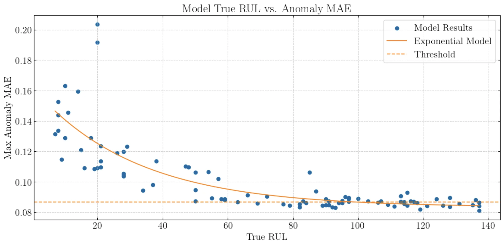
An example of an exponential fit and the MAE vs. RUL graph, with a Spearman correlation of -0.8.
Detecting Faults
When training our LSTM on the jet engine data, our LSTM has a baseline “reconstruction error”. Based on the way we handled the data, we can take this error as the reconstruction error caused by normal operation of a healthy, pre-fault engine. We then define a 97.5% threshold from this value, a safe way we can claim the development of a fault in an engine. We need to examine the distribution of the errors to know for sure. For example, the mean error could be caused by a normal distribution, or by a bimodal distribution with peaks very far apart.
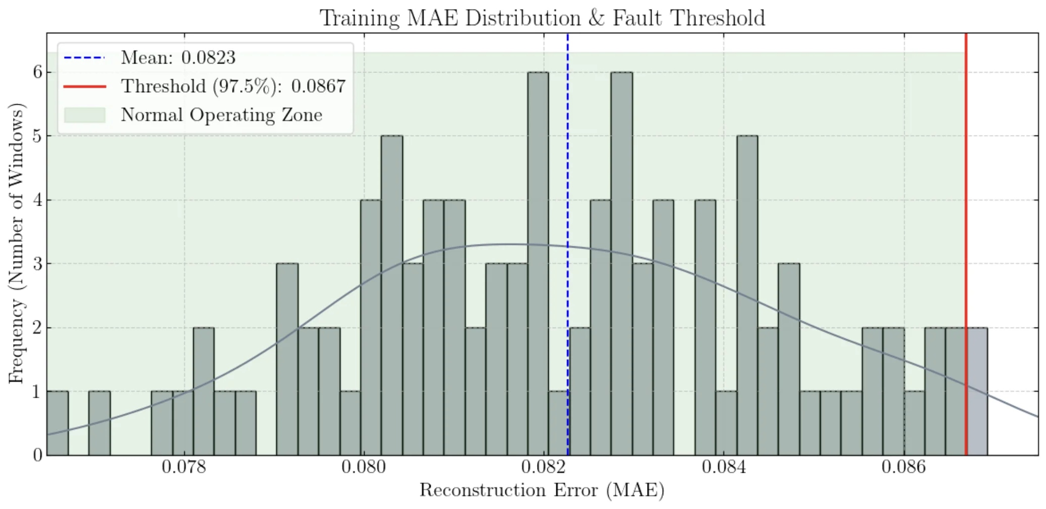
Error distribution of the training set based on healthy engines.
From the above example image, we can see that the errors are well-distributed around the mean, so the 97.5% threshold is a safe value to use.
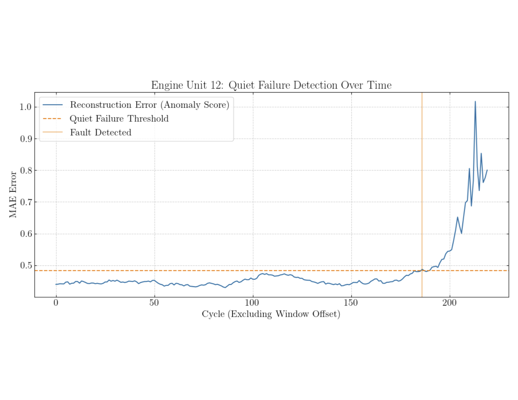
Now, with test data, we can have the LSTM take in the test data, and return the reconstruction loss per timestep (or window). Then, we can check if this error ever surpasses this reconstruction loss threshold, which if it does, we can claim a fault has occurred (like in the image below).
An example of a fault being detected at a cycle of about 180.
More
For more details an explanation, see the project file or the presentation PDF.
